Writing 9 min read
The apical hook, one cell at a time
Rebuilding our 2024 hook model cell by cell, with stress emerging from a force balance rather than prescribed. It confirms the wall-integrity hypothesis under a harder test — and turns up a feedback the analytic version cannot have.
In Walia, Carter et al. (2024) we argued that the Arabidopsis apical hook opens because cell wall anisotropy is dynamic: cortical microtubules follow the maximal principal stress, cellulose follows the microtubules, and the wall is therefore stiffest along the direction it is most loaded. The hook's toroidal geometry does the rest — it puts more hoop stress on the inner side than the outer, so as sub-epidermal growth loads the organ longitudinally, the outer flank's microtubules flip to longitudinal before the inner flank's do.
The model behind that argument is analytic. The hook is a torus, resolved into a handful of independent parts at chosen angles, and each part's stresses come from closed-form thin-walled-vessel expressions:
def calc_long_stress(self) -> None:
    factor = self.par.p * self.par.r / (2 * self.par.t)
    self.long_stress = factor + self.par.long_internal_stress_rate * self.time
That is a deliberate choice and it buys a great deal: the model is fast, it is transparent, and every term in it can be reasoned about on paper. But it means stress is an input. It does not depend on what the tissue does in response.
I have spent the last while rebuilding the thing cell by cell, as a real mechanical object, mostly to find out what that assumption was hiding.
The rebuild
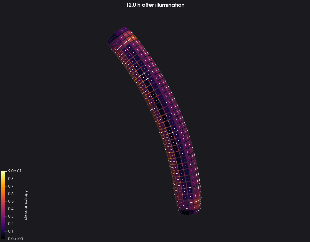
The new version is a vertex model: the hypocotyl epidermis as a closed, turgid, centre-triangulated shell of 514 cells, with proper 2D wall elasticity via triangular biquadratic springs. Walls yield irreversibly above a Lockhart threshold. Turgor acts normal to the shell. The whole thing runs on a ground-up rewrite of Tissue in modern C++, which is a separate story.
The important difference is not the cell resolution. It is that stress is now an output. Nothing prescribes it; it emerges from the force balance of a deformable surface under pressure, and every growth event changes it.
First, does the geometry still hold up?
Before anything else: the analytic model's central geometric claim is that hoop stress varies around the hook as
sigma_hoop ∝ (2λ + sin φ) / (λ + sin φ)
which at our fitted λ = 2.88 gives 2.53× the reference on the inner flank and 1.74× on the outer — a ratio of 1.454.
Measuring the maximal principal stress directly in the cell-resolved shell, on a mesh that was never fitted to that expression, gives an inner/outer ratio of 1.460. Agreement to 0.4%.
That is a good result for the original model and worth stating plainly. The thin-walled toroid is an excellent description of the stress field in a cell-resolved, mechanically consistent shell. The geometry was never the question.
What was missing
The loading was. A vertex model of the epidermis alone represents everything inside it as a uniform turgor pressure, so the only longitudinal load is the pressure-vessel term. With nothing stretching the epidermis along the organ axis, the hoop direction always wins and no switch ever occurs — which is a useful negative result in itself, since it says the switch cannot come from turgor and geometry alone.
Adding it is not simply a matter of applying an axial force, and two constraints make that clear.
A prescribed tension along the axial walls does raise longitudinal stress, but tension along the surface of a curved shell exerts a straightening moment: the load needed to flip the anisotropy opens the hook 23° in three minutes. The analytic parts are immune to this, because each carries a prescribed stress with no coupling to the organ's shape.
Nor can the epidermis simply be held short of its own reference length. With growth switched off so that nothing relieves it, both principal stresses fall over two hours — a shell free to contract simply contracts until strain re-equilibrates against turgor.
What the inner tissue provides is a body the epidermis cannot contract past. So it is modelled as a core with its own reference length per axial wall, which grows proportionally — a similarity transform, so curvature is preserved and no straightening moment appears — and pushes one-sidedly, resisting compression but never pulling. Being one-sided also makes it a floor rather than a constraint: the inner flank can outgrow it, while the outer flank is held stretched against it.
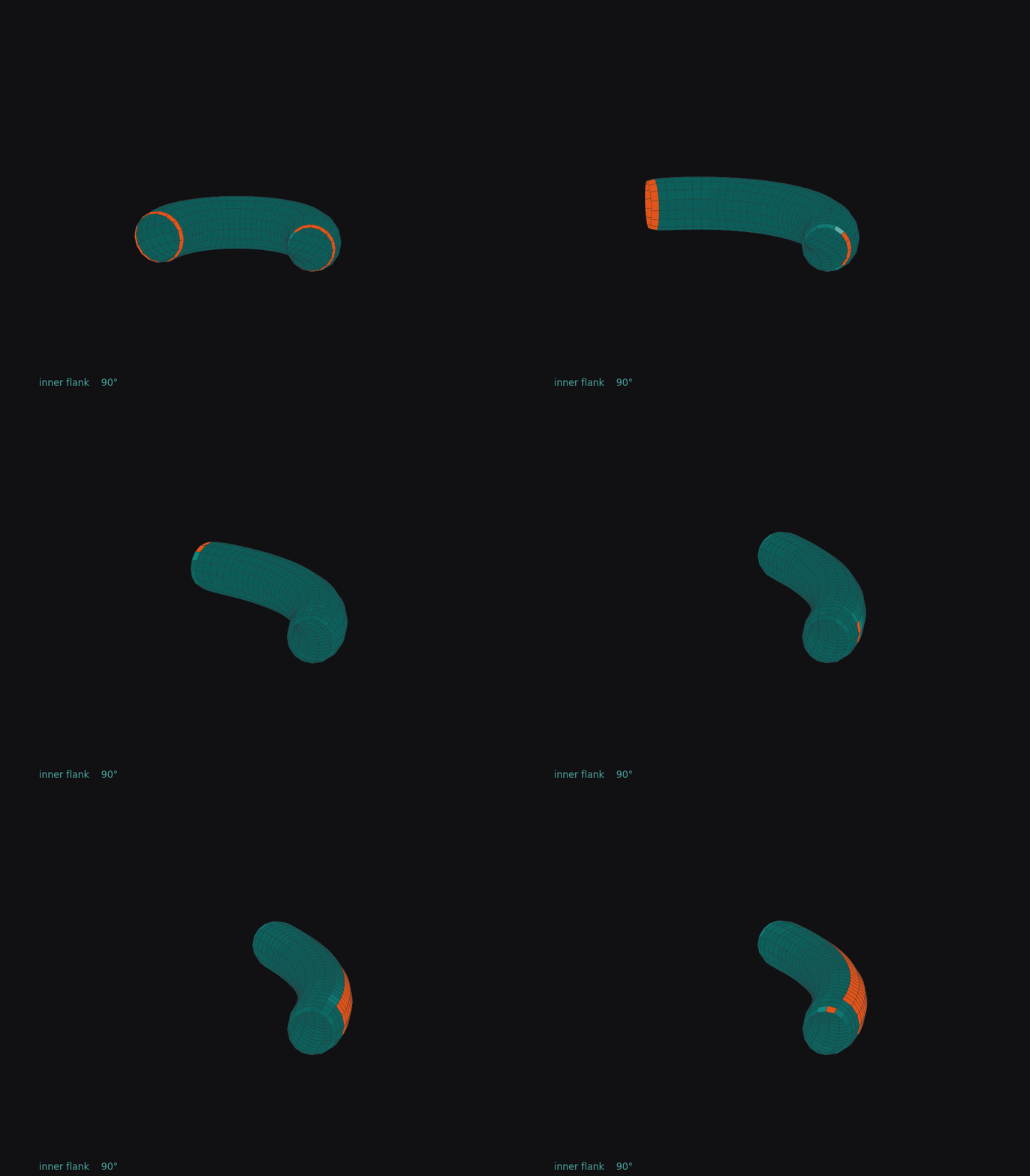
With that in place the switch appears, at true mechanical equilibrium.
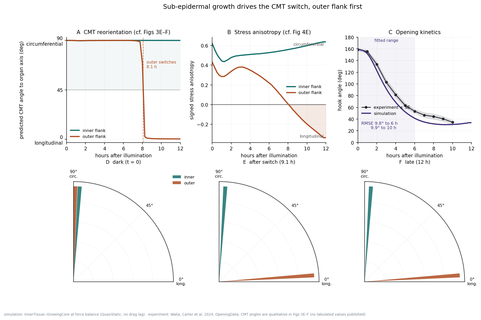
hook_part.py — positive when hoop dominates, negative when
longitudinal does — so the switch is a zero crossing, directly comparable
with Figure 4E of the paper.
Opening kinetics come out at RMSE 9.9° over ten hours. For context, the same model integrated as overdamped dynamics — which lags behind force balance — managed 11.9°. Making the mechanics honest improved the fit.
A thing only this version can produce
The analytic model gives three curves, one per part. A cell-resolved model gives a switch time for every cell, which makes the switch a map rather than a summary.
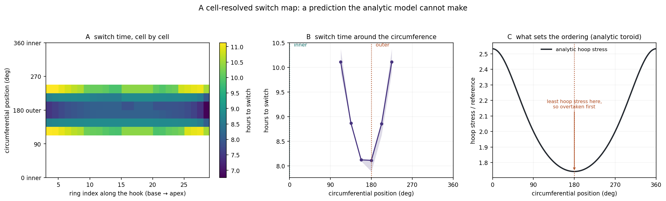
This is a testable prediction rather than a restatement. It says the switch should not appear simultaneously across the outer flank but spread around the circumference over roughly four hours, with a front whose shape follows the hoop-stress curve. Per-cell CMT imaging of the kind already in the paper could be re-analysed against it.
Isoxaben and wall-integrity compensation
Cellulose synthesis inhibition slows hook opening, which looks at first like a problem for any Lockhart model: lowering fibre stiffness softens the wall, and a softer wall yields faster. The sign is forced by the growth law.
But reduced cellulose is not the whole treatment. Our prescription is low Y_f
plus a compensatory Y_m increase plus raised longitudinal stress, on the
grounds that low-dose isoxaben triggers cell wall integrity signalling and
matrix reinforcement — feronia and the1-4 mutants are hypersensitive to it.
Running that here, against lowering Y_f alone as a control:
| variant | Y_f |
Y_m |
core rate | opened by 5 h | outer switch |
|---|---|---|---|---|---|
| mock | 1350 | 20000 | 0.025 | 108.3° | none |
Y_f only |
470 | 20000 | 0.025 | 110.4° | none |
| full prescription | 470 | 30000 | 0.04 | 63.5° | 3.0 h |
| stronger compensation | 470 | 40000 | 0.05 | 35.4° | 1.25 h |
Opening slows by 41%, and the CMT switch accelerates from never-within-the-run
to three hours — both effects reported experimentally, with the dose-dependence
going the right way on both. Lowering Y_f alone does neither.
That is a stronger test than the analytic model can give, because here the longitudinal stress is not prescribed: it emerges, and growth is continuously relieving it. The compensation mechanism survives that.
The finding I did not expect
Here is the one that seems genuinely new.
Our fitted stiffness ratio is Y_m : Y_f = 75 : 100 — the fibre carries about
57% of the wall's load. That share turns out to be the most consequential
parameter in the whole model, and not in the direction I expected.
The argument for raising it is straightforward. Stress scales with applied load; strain scales with load over stiffness. The outer flank has to carry enough longitudinal stress to flip the anisotropy while extending only 1.055×, which is what a stiff wall delivers. So a fibre carrying 57% rather than a few percent should make the model better on both counts at once.
Half of that holds. At the published ratio the strains come out almost exactly right — outer flank 1.065× at eight hours against 1.055× measured, inner flank 2.075× against 2.149×.
The other half does not. At the published stiffness ratio the switch never happens at all, at any core rate.
The reason is a feedback loop that the analytic model cannot contain. Equation 3 stiffens the wall along the maximal-stress direction. A stiffer direction carries its load at lower strain. The two principal strains therefore equalise, and the anisotropy that drove the redistribution falls. Measured at matched times:
| t (h) | fibre 2.7% of load: inner / outer | fibre 57%: inner / outer |
|---|---|---|
| 0.5 | 0.510 / 0.328 | 0.499 / 0.152 |
| 1.0 | 0.443 / 0.284 | 0.516 / 0.195 |
| 2.0 | 0.477 / 0.336 | 0.509 / 0.187 |
| 3.0 | 0.499 / 0.380 | 0.430 / 0.144 |
And the damping is selective, which is what makes it bite. The inner flank is
untouched — it sits where g(a) is near saturation, so the redistribution is
near its limit whatever the fibre share. The outer flank halves, because it sits
on the steep part of the Hill curve. The outer flank is, of course, the one
whose switch the mechanism exists to explain.
In the analytic model this loop cannot close: calc_hoop_stress and
calc_long_stress depend only on pressure, geometry and time, and the
stiffnesses computed from the anisotropy feed forward into growth without ever
altering the stress. There, anisotropy is an input to the material law. Here it
is also an output of it, and the law fights itself.
So the constraint is this. Reproducing a sharp outer-flank switch in a mechanically self-consistent model requires either a smaller fibre contribution than the nominal ratio, or a CMT response that saturates or carries hysteresis so that reorientation is not undone by the stress relief it causes.
Both are testable, and neither is evidence against the mechanism. The switch, its inner/outer ordering, and the isoxaben compensation all reproduce here — at a lower fibre share. What the cell-resolved version adds is that the mechanism's own feedback places an upper bound on how much of the wall's load the microtubule-guided fibre can carry, and the published ratio sits above it.
There is a tension in the model worth naming, because the two halves of that result pull against each other: the stiffness that gets the strains right is the stiffness that kills the switch. Something has to give, and finding out what would be the obvious next experiment.
Caveats, which are not small
The parameters here are hand-tuned, not jointly fitted, and single configurations have not been repeated. The growing core's stiffness and rate are set by hand. And the whole exercise rests on a re-implementation: where it differs from the published model, the difference usually reflects a modelling choice made here rather than an error there.
One discrepancy I want to leave standing rather than explain away. The inner flank never switches in my runs, in twelve hours, at any parameter set I tried — where we report that it does, later than the outer. In this model the inner flank's hoop stress is simply too far ahead: at the moment the outer flank crosses over, its two principal stresses differ by 2%, while the inner flank's still differ by a factor of 2.3 and are not converging. Either the inner switch needs something my version lacks, or its reorientation is driven by something other than the instantaneous principal stress direction. I do not know which, and it is the question I would most like answered.
Code
The rewritten simulator, the hook model, the analysis scripts and everything
needed to regenerate these figures are in the v2/hypocotyl directory of my
Tissue fork. The reactions that matter for this post are
VertexFromTRBScenterTriangulation (the stress solver),
WallMechanics::FiberSpring (Equation 3), WallGrowth::AcidGrowth, and
InnerTissue::GrowingCore.